Final project report part 2: overview

Overview

I am very happy with the outcome of my work at GSoC. On the one hand it is true that the complete list of goals in the original application has not been accomplished. On the other hand, the focus of contributions changed once I started working. I implemented a lot of observation handling code that was not already available as planned, instead of background model application to source observations. Indeed, the majority of the items in the API proposal have been worked out and added as functionality to Gammapy. In addition, I participated in the necessary code cleanup for the release of Gammapy version 0.3.

List of main pull-requests during my GSoC (all merged in the trunk):

• Document observation tables and improve gammapy.obs [#278]
• Observation table subset selection [#295]
• Add cube background model class [#299]
• Make background cube models [#319]

Other relevant pull-requests (also merged):

• Add function to fill acceptance image from curve [#248]
• Consistent random number handling and improve sample_sphere [#283]

(There are more (smaller) pull-request dealing with cleanups, fixes or small additions that are not listed here.)

All in all, a lot of new functionality has been successfully added to Gammapy, as demonstrated by the example in the example section in the final project report part 1 post, and the examples in the documentation links listed below, making this a fruitful project.

As summary of my work produced during the GSoC, I am repeating the list of links to the documentation I produced during the GSoC, that I already posted in the progress section in the final project report part 1.
This documentation explains the most important contributions produced during my GSoC project:

• observation lists format and generation.
• dataset generation.
• observation selection.
• observation grouping.
• cube background models.
• cube background model production.

I would like to take the opportunity to thank the mentors of the project for their useful input. There was at all times at least one of them there to answer my questions and give positive feedback. I learnt a lot during this summer!

For instance I deepened my knowledge of the scientific python stack: numpy, scipy, matplotlib. I learnt of course the basic tools needed for my project: git, GitHub, Astropy, Gammapy. I also learnt how to work collaboratively in a pull-request system with code reviews.

These recently acquired knowledge, together with my previous skills in programming with object-oriented languages granted me access to the list of Gammpy core developers and maintainers with write access to the repository.

To conclude, the completion of this works has taken many hours of hard work (~ 500 h), much satisfaction, some frustration and 0 drops of coffee! :-)

Final project report part 1: progress

The last 2 weeks of Google Summer of Code (GSoC) have been a bit intense and exciting.

Gammapy 0.3

First of all Gammapy version 0.3 has been released. It is still an alpha version of Gammapy. But it contains already some of the functionality I developed for the GSoC. For instance:

• dummy observation table generator.
• container class for cube data.
• dummy background cube model generator.
• observation selection tools.
• many small fixes.

Progress

As for my work on the last 2 weeks, I spent much of the time refactoring the code of the background cube model production script mentioned in my previous report and integrating the functionality into Gammapy. In addition, I added some tests
to assure that the recently added code works, and documented the new classes, methods and scripts.

New functionality added to Gammapy:

• Observation grouping classes: classes to define groups of observations with similar properties (like observation altitude/azimuth angle or number of telescopes participating in the observations) in order to be analyzed in groups instead of individually
• Format converters: methods to convert the observations list formats of different experiment into the Gammapy observation list format.
• Dummy dataset generator: methods to generate a dummy dataset with event lists (data) and effective area tables (instrument response functions) in order to test some of the Gammapy functionality. The tools work as follows:
• generate a dummy observation table, generated with the tool mentioned above.
• Simulate background data (using a very simple model) according to the produced observation table
• Store the data emulating the data structure of an existing experiment, like H.E.S.S..
• Class to handle the creation of background cube models: the methods acting on background cube models have been divided into 2 classes:
• Cube: the basic container class for cube data mentioned above. This class is kept as generic as possible, allowing other classes to use it to contain other kinds of cube data in the future. It contains basic I/O functionality, plotting methods, and methods operating on the cubes.
• CubeBackgroundModel: class with methods specific for the background cube model productions, such as binning, histogramming, and smoothing. It also defines 3 cubes necessary for the model production:
• counts cube: contains the statistic participating in the model.
• livetime cube: contains the livetime correction to apply.
• background cube: contains the model.
• Command line tool to run the production of background cube models: this tool takes as input a dataset either from an existing experiment like H.E.S.S., or simulated data produced with the tools mentioned above and produces the models in several steps:
• Produce a global observation list, filtering observations taken close to known sources. The tool selects all observations far from the sources listed in the TeVCAT catalog.
• Group the observations according to similar observation properties, in this case: altitude and azimuth angles.
• For each group produce the background cube models by:
• define binning.
• fill events and livetime correction in cubes.
• fill events in bg cube.
• smooth the bg cube to reduce fluctuations due to (low) Poisson statistics.
• correct for livetime and bin volume.
• set 0 level to something very small.
• Example script to make a few plots comparing 2 sets of background cube models.
• Added a new file to gammapy-extra with a test CubeBackgroundModel object

More details on the background cube model production can be found online in the documentation I produced during the GSoC, especially in the last week:

• observation lists format and generation.
• dataset generation.
• observation selection.
• observation grouping.
• cube background models.
• cube background model production.

Example

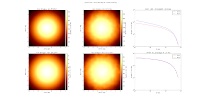
As an example of the new capabilities of Gammapy in order to produce background models, I produced 2 different models using the tools I developed and documented here and compared them:

• A simulated background cube model (a.k.a. true model).
• A reconstructed model (a.k.a. reco model) using simulated data following the model used for the true model.

The models very roughly represent the background seen by a H.E.S.S.-like experiment at an altitude close to the zenith and South azimuth.

Using the example script to plot 2 models together for comparison I produced the following plot (click for an enlarged view):

The plot shows that the reconstructed (reco) model agrees quite well with the simulated (true) model.

The following animated image shows the data of the reco model (click for an enlarged view):

Each frame represents one energy bin of the model, ranging from 0.1 TeV to 80 TeV. The pictures represent the (X, Y) view of the model in detector coordinates (a.k.a. nominal system), covering a 8 x 8 square degree area.

It is shown that Gammpy can be now used to produce accurate background cube models.

Progress report

My work on the last 2 weeks has been mainly focused in the Gammapy tools to select observations from an observation list that were introduced in the mid-term summary report, and on the script to produce cube background models presented in the last progress report. The progress on these 2 topics is presented in more detail in the following sections.

In addition, I also contributed to some of the clean-up tasks in order to prepare for the release of the Gammapy 0.3 stable version in the coming weeks.

Observation selection

I restructured the code in that I produced a few weeks ago to make it clearer and defined 3 main observation selection criteria:

• Sky regions: these methods select observations on a certain region of the sky, defined as either a square (sky_box), or a circle (sky_circle).
• Time intervals: this method selects observations in a specific time range, defined by its minimum and maximum values.
• Generic parameter intervals: this method selects observations in a (min, max) range on a user-specified variable present in the input observation list. The only requirement for the variable is that it should be castable into an Astropy Quantity object: the variable should represent either a dimensionless quantity (like the observation ID), or a simple quantity with units (like the altitude angle or the livetime of the observations).

More details are given in the documentation I wrote for the select_observations function.

In addition I produced a working inline-command tool to act on an input observation list file and output a selected observations file. This tool can perform the same kind of selections mentioned above in a recursive way. More details are given in the documentation I wrote for the gammapy-find-obs tool, that uses the find-obs script.

In order to test the gammapy-find-obs tool, a dummy observation list file produced with the make_test_observation_table tool presented in the first report has been placed in the gammapy-extra repository here.

Cube background model production

I produced a working version of the script that produces cubes similar to the one presented in the animation on the last post with many improvements.

The new version of the script uses a finer binning both in altitude/azimuth angles for the observation grouping, and in (X, Y, energy) coordinates for the cube itself. The binning on (X, Y, energy) also depends on the amount of statistics (coarser coordinate binning for observation groups with less statistics)

In addition, a smoothing to avoid Poisson noise due to low statistics is applied to the background cube model. The smoothing also depends on the available statistics: cubes with more statistics are smoothed less than cubes with less statistics. The smoothing applied is quite simple. It is performed by convoluting the 2D image of each energy bin of the cube independently with a certain kernel, and scale the smoothed image to preserve the original integral of the image. The kernel chosen is the default kernel used by the ROOT TH2::Smooth function: it is named k5a and acts on 2 layers of surrounding pixels (i.e. 2 next neighbors). Interpreting images as 2D arrays, the kernel is represented by the following matrix:

0 0 1 0 0

0 2 2 2 0

1 2 5 2 1

0 2 2 2 0

0 0 1 0 0

I applied the script to the H.E.S.S. data to produce background models for a full set of altitude/azimuth angle bins with satisfactory results. Unfortunately, since the data is not public, I am not allowed to post any figures or animations showing them.

The current version of the script is functional but still a bit chaotic, because it consists of only a few long functions. Therefore, the next steps, to be accomplished in the remaining time of the Google Summer of Code, is to integrate the script into Gammapy, refactorize the code and move most of its functionality into methods and classes within Gammapy.